
Multilayer Perceptron
A Multilayer Perceptron is a connected collection of individual Perceptrons capable of solving more advanced problems than a single Perceptron. They are organized by layers, each feeding their output as an input into each perceptron in the next layer.
Each Perceptron is considered a Neuron and this structure is considered as a Neural Network. We will be working through a Supervised, Fully Connected, Feedforward Neural Network.
Problem with Perceptrons
A Perceptron is limited in what it can solve. They can only solve "linearly separable" problems, meaning the classification between our answers can be divided with a single line. This was our Perceptron example where we were literally classifying points around an arbitrary function as either on one side of a line or another.
Consider the problem of identifying a number within a picture. We would want our Perceptron to have an input for each pixel of the image, in a 20x20 image that would be 400 inputs. We need the Perceptron to give us a probability of what digit it is, one probability per digit. So we would have 10 outputs.
If we look at boolean OR and boolean AND and we create a table for them, we can see that both OR and AND can be linearly separable and therefore solved by our Perceptron.
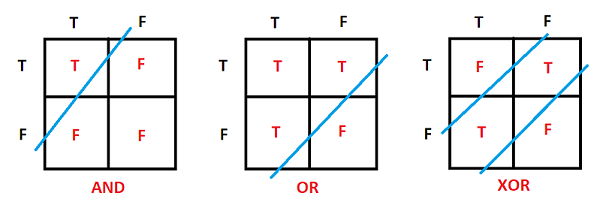
However for XOR boolean operations we cannot linearly separate them and therefore XOR cannot be solved by a single Perceptron.
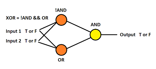
If we break down what XOR is, we can see it it is the combination of AND and OR: XOR = !AND && OR. Therefore we could train one perceptron on !AND, another on OR and feed their inputs to a third trained on AND. These connected Perceptrons would produce a correct XOR answer.
Fully Connected, Feed Forward Neural Network
To generalize a Neural Network in code, we want to create: an input layer with a number of input neurons, a hidden layer with a number of hidden neurons, and an output layer with the number of output neurons.
Example: new NeuralNetwork(input=2, hidden=3, output=2);
In a Fully Connected network every preceding layer's neurons are connected to every successive neighboring layer's neurons. So with 2 input neurons, each one sends its outputs to every hidden neuron so in total there are 6 connections. Then each hidden neuron sends its output to each output neuron.
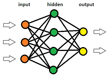
More advanced Neural Networks have several hidden layers, not just one, in order to process more complicated problems.
In a Feed Forward network each neuron will do a weighted sum of the incoming data and weights. So for our 2/3/2 NN a single hidden neuron will have two connections of data coming in as inputs. Each connection has its value and its weight and it will multiply each value times its weight and add them to each other input's. sum = x1 * w1 + x2 * w2 + ... xN * wN. See the Perceptron doc for more detail.
Once the weighted sum is calculated in the neuron, it is passed through the "activation function" (see perceptron.md) and the output is passed on to the next layer as inputs.
Modeling with a Matrix
An obvious approach to modeling this structure would be to model each neuron as an object and each connection to the neuron as another object. At that stage you could pass data forward through neurons doing calculations one by one. But the standard approach to modeling the data as it passes through a network is to use a Matrix.
A simpler example we can break down:
NN (2 inputs, 2 hidden, 1 output)
If x1 is fed into the first input, and x2 is fed into the second input, and its a fully connected feed forward network then we can use linear algebra to calculate the sums of the hidden layer.
            w11
x1 -> ( i1 )---( h1 )
            \/w12   \
            /\       >--( o1 )
           /  \w21  /
x2 -> ( i2 )---( h2 )
            w22
Weights:
- w1-1 is the weight from input 1 to hidden 1
- w1-2 is the weight from input 1 to hidden 2
- w2-1 is the weight from input 2 to hidden 1
- w2-2 is the weight from input 2 to hidden 2
Matrix Notation:
(w11 w21) * (x1) = (h1)
(w12 w22)   (x2)   (h2)
We have a 2x2 matrix of weights and a 2x1 matrix of inputs (rows by cols).
We need a weighted sum as seen with our perceptron. h1 sum = x1 * w11 + x2 * w21 and h2 sum = x1 * w12 + x2 * w22.
These summations are linear algrebra of matrix multiplication.
See the neural network linear algreba doc on matrix mathematics used to calculate our weighted sums through a dot product.
The Feedforward Algorithm for Guessing
With our understanding of a Perceptron and a Multilayer Perceptron structure, we understand that each neuron will calculate the weighted sum of its inputs and their connected weights.
What we can use is matrix mathematics to perform this math for us to multiply a weight matrix by the input matrix to recieve the sums of our neurons (before the activation function).
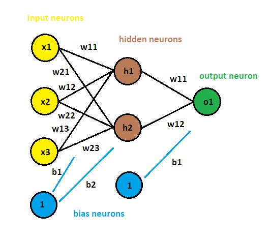
An example with 3 input neurons, 2 hidden neurons and 1 output neuron:
- There are 3 Input neurons: x1, x2, x3
- There are 2 Hidden neurons: h1, h2
We want to organize our weights by their hidden neuron and their input neuron.
- There are 6 weights: w11 for h1-x1, w12 for h1-x2, w13 for h1-x3, w21 for h2-x1, w22 for h2-x2, w23 for h2-x3
If we model the weights of our neurons as a matrix we should see:
W = [ w11 w12 w13 ]  2x3 matrix
    [ w21 w22 w23 ]
Then we want to model our input neurons with a matrix, one row per input:
X = [ x1 ]  3x1 matrix
    [ x2 ]
    [ x3 ]
We can take the Dot Product of these two matrices because the columns in the weight matrix are the same as the number of rows in the input matrix.
NOTE we organize the weights by hidden-to-input and then create the input matrix second because thats the only way to get the matrices to be a 2x3 dot 3x1.
dot product of weights
W . X = H
[ w11 * x1 + w12 * x2 + w13 * x3 ] = [ h1 ]
[ w21 * x1 + w22 * x2 + w23 * x3 ] = [ h2 ]
Including the Bias
In our Perceptron model we recognized the limitation of dealing with 0 value inputs because the weights would always calculate as 0. To overcome this we introduced a bias that was added against the weighted sum to always prevent a zero summation.
If H = W . X (hidden values equal weight matrix dot product the input matrix), we need to add our bias into that. That becomes H = W . X + B where B is the bias matrix.
We would have one bias value per hidden neuron so:
B = [ b1 ]  1x2
    [ b2 ]
and
W . X = S
S + B = H

dot prduct
[ w11 * x1 + w12 * x2 + w13 * x3 ] = [ s1 ]
[ w21 * x1 + w22 * x2 + w23 * x3 ]   [ s2 ]

element-wise addition
[ s1 ] + [ b1 ] = [ h1 ]
[ s2 ]   [ b2 ]   [ h2 ]

[ s1 + b1 ] = [ h1 ]
[ s2 + b2 ]   [ h2 ]
Include the Activation Function as the Sigmoid Function
The Sigmoid Function is a function that has the characteristic of an "S" or sigmoid curve. On a cartesian coordinate the lower left of the S would start at about -6,0, the center point would be 0,0.5 and the upper right would be at about 6,1. We can see that the x range is hyperbolically between -6 and +6 and the y from 0 to 1.
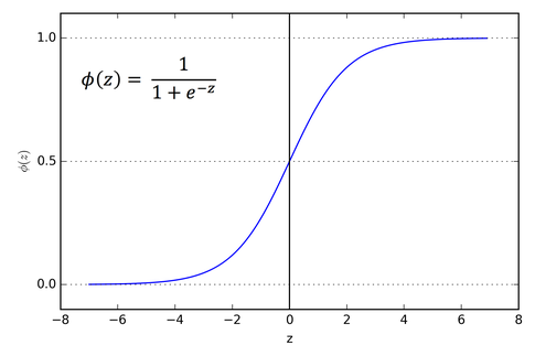
S(x) = f(x) = 1 / (1 + e^-x)
It is used in neural networks because if you pass any number into the sigmoid function you will get a number between 0 and 1.
Using the sigmoid function as an activation function our final hidden output calculation becomes the weight matrix dot input matrix plus bias matrix passed through the sigmoid function.
H = Sigmoid( W . X + B )
Our Final Output Layer
Now that we have the hidden layer outputs calculated, those outputs become the inputs for the final output neuron. The same feed forward algorithm is applied.
- Create our weighted matrix from output neuron mapped to input value
- Create our input matrix, each input per row
- Create our bias matrix, a bias per output neuron (1)
- Calculate the dot product and element-wise addition of these matrices
- Pass the result through the sigmoid function
Programming our Feedforward Guessing
Our ultimate objective is the implementation of a Neural Network that appears as such:
let nn = new NeuralNetwork(2, 2, 1); // input, hidden, output
let input = [1, 0];
let output = nn.feedforward(input);
class Matrix {
// see linear algebra doc for implementation examples
// transpose()
// randomize(min, max)
// elementWiseAdd(m)
// elementWiseMultiply(m)
// elementWiseSubtract(m)
// scalarAdd(n)
// scalarMultiply(n)
// scalarSubtract(n)
// map(func)
// print()
// static dotProduct(a, b)
// static fromArray(a)
// static toArray(a) (cols->rows)
// static clone(m)
}function sigmoid(x) {
return 1 / (1 + Math.exp(-x));
}class NeuralNetwork {
// 3 Layer
constructor(inputNodes, hiddenNodes, outputNodes) {
this.inputNodes = inputNodes;
this.hiddenNodes = hiddenNodes;
this.outputNodes = outputNodes;
// Create our weight matrix, input as columns, hidden as rows
this.weights_ih = new Matrix(this.hiddenNodes, this.inputNodes);
// Create our second weight matrix, hidden as columns, output as rows
this.weights_ho = new Matrix(this.outputNodes, this.hiddenNodes);
// Get some random weights from -1 to 1
this.weights_ih.randomize(-1, 1);
this.weights_ho.randomize(-1, 1);
// Create our biases
this.bias_h = new Matrix(this.hiddenNodes, 1);
this.bias_o = new Matrix(this.outputNodes, 1);
this.bias_h.randomize();
this.bias_o.randomize(); // isnt this risky if = 0?
}
// Creates a weighted guess
feedforward(inputArray) {
// As a convenience convert an array to a Nx1 matrix
let inputs = Matrix.fromArray(inputArray);
// Calculate the dot product of the weights and inputs
let hiddenLayerOutput = Matrix.dotProduct(this.weights_ih, input);
// Element wise add the bias
hiddenLayerOutput.elementWiseAdd(this.bias_h);
// Map an activation function
hiddenLayerOutput.map(sigmoid);
// Repeat steps for output layer
let outputLayerOutput = Matrix.dotProduct(this.weights_ho, hiddenLayerOutput);
outputLayerOutput.elementWiseAdd(this.bias_o);
outputLayerOutput.map(sigmoid);
// Return output
return Matrix.toArray(outputLayerOutput);
}
}In our code examples we have a Neural Network that utilizes matrix math and three (hardcoded) layers to create weighted guesses against a series of inputs.
Lets continue this by looking back at how to train our Neural Network with a Backpropagation algorithm.
The Backpropagation Algorithm for Training
Utilizing Supervised learning we are going to train our Neural Network through backpropagation of error.
In our Perceptron training we calculated the error as:
error = answer - guessdelta(weight) = error * inputnew weight = weight + ( delta(weight) * learningRate )
With these steps we incrementally adjusted the weight by adding the how much it was incorrect. To prevent oversteering we introduced a learning rate so its error adjustment was not too extreme.
In our multilayer perceptron when we have multiple neurons responsible for producing incorrect output we must adjust the weights of the neurons individually. We cannot wholesale update each neuron with the same error calculation as one neuron would need more adjustment than another.
Proportional Adjustment Problem
If we have two neurons that have fed a single output neuron which had an incorrect error, we would need to adjust the weight of each neuron individually.
Let
ybe our output andy = .7- our correct answer was
1 - we have 2 hidden inputs,
h1, h2 - weight from
h1to output was.2 - weight from
h2to output was.1 - we could say that
h1is 67% responsible andh2is 33% responsible
But what about if we have even more layers? We may be able to calculate our error on the output and adjust the weights of incoming neurons, but we must also adjust the weights of every preceding neuron in the neural network. So we must adjust the weights individually by calculating the error at each neuron and adjusting the weights of the preceding and connected neurons.
We must know how to calculate our error at each neuron and back-propagate adjustments.
Let's breakdown how we would calculate a single layer's error adjustment.
Let
`h1` be hidden neuron 1
`h2` be hidden neuron 2
`o1` be output neuron
`w1` be weight from `h1` to `o1`
`w2` be weight from `h2` to `o1`
`eh1` be error of hidden neuron 1
`eh2` be error of hidden neuron 2
`eo1` be error of the output neuron
`g1` be the guess
`a1` be the answer
If
`a1 = 1`
`g1 = .7`
`w1 = .2`
`w2 = .1`
Then
`eo1 = .3`
`eh1 = ( w1 / ( w1 + w2 ) ) * eo1 = .2`
`eh2 = ( w2 / ( w1 + w2 ) ) * eo1 = .1`
Lets introduce another output neuron so we can see how complicated it becomes with more than one output neuron feeding back an error to the connected weights.
Let
`h1` be hidden neuron 1
`h2` be hidden neuron 2
`o1` be output neuron 1
`o2` be output neuron 2
`w11` be weight from `h1` to `o1`
`w21` be weight from `h1` to `o2`
`w12` be weight from `h2` to `o1`
`w22` be weight from `h2` to `o2`
`g1` be guess for output 1
`g2` be guess for output 2
`a1` be correct answer for output 1
`a2` be correct answer for output 2
`eo1` be error of the output neuron 1
`eo2` be error of the output neuron 2
`rh11` be the hidden 1 percentage of responsibility for error 1
`rh21` be the hidden 1 percentage of responsibility for error 2
`rh21` be the hidden 2 percentage of responsibility for error 1
`rh22` be the hidden 2 percentage of responsibility for error 2
`eh1` be error of hidden neuron 1
`eh2` be error of hidden neuron 2
If
a1 = 1
a2 = 0
g1 = .7
g2 = .4
w11 = .2
w21 = .1
w12 = .5
w22 = .3
Then we calculate error for each hidden node. It is the percentage of error responsibility times the error plus summed for all ouptut nodes.
eo1 = ( a1 - g1 ) = .3
eo2 = ( a2 - g2 ) = -.4
rh11 = ( w11 / ( w11 + w12 ) ) * eo1 = 0.0857142857142857
rh21 = ( w21 / ( w21 + w22 ) ) * eo2 = -0.1
rh12 = ( w12 / ( w11 + w12 ) ) * eo1 = 0.2142857142857143
rh22 = ( w22 / ( w21 + w22 ) ) * eo2 = -0.3
eh1 = rh11 + rh21 = -0.0142857142857143
eh2 = rh12 + rh22 = -0.0857142857142857
Using this example we have calculated the error for 2 hidden neurons connected to 2 output neurons. We can then take the error for each hidden neuron and run the same calculations to get the error for each neuron in the preceding layer.
This is backpropagation of errors by the gradient descent algorithm.
Reducing Complexity and using Matrix Math
If we look at how the error is calculated we are essentially normalizing each weight by w1 / (w1 + w2). It is possible to not perform the normalization in this step and do it after we have calculated the errors. This allows us to use a Matrix dot product to calculate the errors.
eh1 = w11 * eo1 + w21 * eo2
eh2 = w12 * eo1 + w22 * e02
Which is
[ w11 w21 ] . [ e01 ] = [ eh1 ]
[ w12 w22 ]   [ e02 ]   [ eh2 ]
Now it seems strange that we have ordered our error calculation weight matrix as we have, but if we look we can see that it is the Transpose of our original weight matrix:
original weight matrix
[ w11 w12 ] transpose -> [ w11 w21 ]
[ w21 w22 ]              [ w12 w22 ]
So we can calculate our errors by element-wise subtraction, then adjust our weights through the transpose of our weight matrix dot product with our errors.
Programming our Backpropagation Training
Continued from our prior NeuralNetwork code.
let nn = new NeuralNetwork(2, 2, 1); // input, hidden, output
let inputs = [1, 0];
let targets = [1]
nn.train(inputs, targets);
function sigmoid(x) {
// ...
}
function derivativeSigmoid(x) {
// If x has not been sigmoided
return sigmoid(x) * (1 - sigmoid(x));
}
function derivative(y) {
// Made this function because we cant use derivativeSigmoid on a value already sigmoid
return y - (1 - y);
}class NeuralNetwork {
// 3 Layer
constructor(inputNodes, hiddenNodes, outputNodes) {
// ...
// Add a learning rate
this.learningRate = 0.1;
}
// Creates a weighted guess
feedforward(inputArray) {
// ...
}
// Trains with error backpropagation
train(inputArray, targetArray) {
let inputs = Matrix.fromArray(inputArray);
let targets = Matrix.fromArray(targetArray);
// RECALCULATE FEEDFORWARD TO GET OUTPUTS
// Like we did with feedforward, we need to calculate our outputs
// Calculate hidden layer first
let hiddenLayerOutput = Matrix.dotProduct(this.weights_ih, input);
hiddenLayerOutput.elementWiseAdd(this.bias_h);
hiddenLayerOutput.map(sigmoid);
// Repeat steps for output layer
let outputLayerOutput = Matrix.dotProduct(this.weights_ho, hiddenLayerOutput);
outputLayerOutput.elementWiseAdd(this.bias_o);
outputLayerOutput.map(sigmoid);
// OUTPUT ERROR ADJUSTMENT TO HIDDEN
// Calculate the error from output layer
// error = targets - outputs
let outputErrors = Matrix.elementWiseSubtract(targets, outputLayerOutput);
// Calculate our output gradient (Gradient Descent Algorithm (need notes on this))
// Delta of Weights H->0 = learningRate * outputErrors * ( outputs * ( 1 - outputs ) ) * transposeHidden
// ^^^^^^^^^ gradient ^^^^^^^^^^
// gradient = outputs * (1 - outputs)
// let gradient = outputLayerOutput * (1 - outputLayerOutput); // assuming sigmoid has set output between 0 and 1
let outputGradients = Matrix.clone(outputLayerOutput);
outputGradients.map(derivative); // we would use derivativeSigmoid but outputs are already sigmoid from above
outputGradients.elementWiseMultiply(outputErrors);
// Calculate our hidden -> output deltas
let transpose_hiddens = this.weights_ho.transpose();
let weights_ho_deltas = Matrix.dotProduct(outputGradients, transpose_hiddens);
// Finally, add our error delta for our weights
this.weights_ho.elementWiseAdd(weights_ho_deltas);
// Calculate output layer bias adjustment which is just the gradient adjustment
this.bias_o.elementWiseAdd(outputGradients);
// HIDDEN ERROR ADJUSTMENT TO INPUT
// Calculate the error from output layer
// error = targets - hidden
let transpose_weights_ho = this.weights_ho.transpose(); // this confuses me
let hiddenErrors = Matrix.dotProduct(transpose_weights_ho, outputErrors);
// Calculate the hidden gradient
// Delta of Weights I->H = learningRate * hiddenErrors * ( hiddens * ( 1 - hiddens ) ) * transposeInput
// ^^^^^^^^^ gradient ^^^^^^^^^^
let hiddenGradients = Matrix.clone(hiddenLayerOutput);
hiddenGradients.map(derivative); // already sigmoid
hiddenGradients.elementWiseMultiply(hiddenErrors);
hiddenGradients.elementWiseMultiply(this.learningRate);
// Calculate our input -> hidden deltas
let transpose_inputs = inputs.transpose();
let weights_ih_deltas = Matrix.dotProduct(hiddenGradients, transpose_inputs);
// Finally add our error delta for our weights
this.weights_ih.elementWiseAdd(weights_ih_deltas);
// Calculate hidden layer bias adjustment which is just the gradient adjustment
this.bias_h.elementWiseAdd(hiddenGradients);
}
}Determining how often to Train
Now that we can guess answers and adjust for errors we need to make a decision on how often to train our network. We could train them "stochastically" with every single input, or we could train in batches. Stochastic training will adjust weights with every input guessed, and batch training will adjust weights every x number of training across the average of errors made.
For this example we will do stochastic adjustment since our code lends itself to that.
Training the XOR Problem
With 2 inputs, 2 hiddens and 1 output we will train our neural network to solve the XOR problem. Our training data will be:
[1, 0] [1]
[0, 1] [1]
[1, 1] [0]
[0, 0] [0]
let trainingData = [
{
inputs: [1, 0],
targets: [1]
},
{
inputs: [0, 1],
targets: [1]
},
{
inputs: [1, 1],
targets: [0]
},
{
inputs: [0, 0],
targets: [0]
}
];
let nn = new NeuralNetwork(2, 2, 1); // input, hidden, output
// Train on our XOR data in a stochastic manner (train on every data input, not an average of a batch)
for (let i=0; i < 1000; i++) {
for (data of trainingData) {
nn.train(data.inputs, data.targets);
}
}
// Test
console.log(nn.feedforward([1, 0]));
console.log(nn.feedforward([0, 1]));
console.log(nn.feedforward([1, 1]));
console.log(nn.feedforward([0, 0]));
This will take a lot of training to show results because we feeding the same order. We can improve it by randomizing the training data coming in.
// Train on our XOR data in a stochastic manner (train on every data input, not an average of a batch)
for (let i=0; i < 1000; i++) {
    let data = trainingData[parseInt(Math.random() * trainingData.length)];
    nn.train(data.inputs, data.targets);
}
I am done.